The Statistics Behind A/B Testing

Most A/B testing tools spit out a confidence percentage and a conversion lift, and most teams treat those numbers as gospel without understanding where they come from. That works fine until you get a result that feels wrong - a “95% significant” winner that doesn’t move the metric in production, or a test that’s been running for weeks and still hasn’t converged. The statistics behind A/B testing aren’t complicated, but they’re precise. Knowing how the numbers are calculated gives you a much better sense of when to trust them and when to push back.

If you are new to A/B testing and want a conceptual overview without the formulas, read How A/B Testing Works first.

Reading an A/B test report#

Before getting into formulas, here’s what a typical A/B test report looks like:

Variation	Conversions / Views	Conversion rate	Change	Confidence
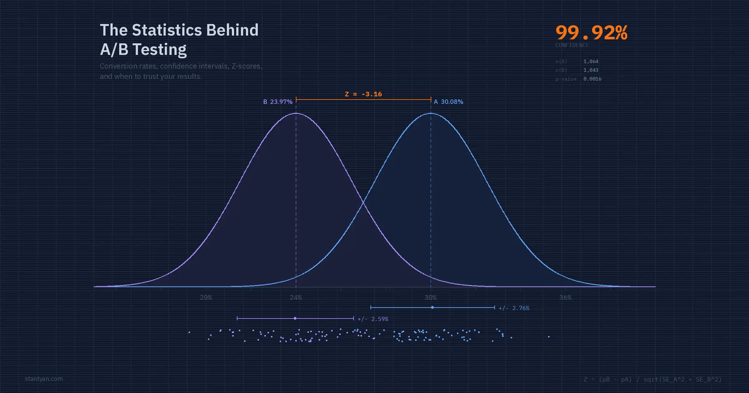
Variation A (Control)	320 / 1064	30.08% +/- 2.32%	-	-
Variation B	250 / 1043	23.97% +/- 2.18%	-20.30%	99.92%

This test has reached statistical significance: confidence is above 95% and both variations have over 1,000 views. Variation B performs worse - its conversion rate is about 6 percentage points lower than the control, and we can be 99.92% confident that this difference is not just random noise.

Every number in that table is calculated from just two raw inputs per variation: a count of conversion events and a count of view events. The sections below walk through each formula, what it means, and how to compute it yourself.

Conversion rate and percentage change#

The conversion rate is the most straightforward metric in the report. It’s the fraction of visitors who did the thing you’re measuring.

For Variation A in the report above: 320 / 1064 = 0.3008, or 30.08%. Simple division, but this is a sample estimate - it’s the conversion rate we observed, not necessarily the true underlying rate. That distinction matters when we get to confidence intervals.

The percentage change tells you how much better or worse the test variation performed relative to the control:

Using the report numbers: (0.2397 - 0.3008) / 0.3008 = -0.2030, or -20.30%. Variation B’s conversion rate dropped by about a fifth compared to the control. But a raw percentage change doesn’t tell you whether the difference is real or just random fluctuation. That’s what the rest of the statistics are for.

Confidence intervals#

A conversion rate calculated from a sample is an estimate, and estimates have uncertainty. If you ran the same test again with a different set of visitors, you’d get a slightly different conversion rate. The confidence interval quantifies that uncertainty - it’s a range around the observed rate where the true rate is likely to fall.

The standard error measures how much the conversion rate would vary across hypothetical repeated samples. For a binomial proportion (which is what a convert-or-not metric is), the Wald method gives us:

This formula has two important properties. First, SE shrinks as the sample size (n) grows - more data means less uncertainty, which should feel intuitive. Second, SE is largest when the conversion rate is near 50% (because that’s the point of maximum uncertainty for a binary outcome) and smallest when it’s near 0% or 100%.

For Variation A: SE = sqrt(0.3008 * 0.6992 / 1064) = sqrt(0.0001977) = 0.01406, or about 1.41%.

The 95% confidence interval multiplies the standard error by 1.96, the critical value for the 95th percentile of the standard normal distribution:

For Variation A: 0.3008 +/- (1.96 * 0.01406) = 0.3008 +/- 0.0276, which gives us 30.08% +/- 2.76%. The report rounds this differently depending on significant digits, but that’s the underlying calculation.

A common misinterpretation: a 95% confidence interval does not mean “there’s a 95% probability the true rate is inside this range.” Technically, it means if you repeated this experiment many times and built an interval each time, 95% of those intervals would contain the true rate. The distinction sounds pedantic, but it matters when you’re deciding how to act on the results. The interval is a statement about the procedure’s reliability, not a probability statement about any single interval.

How sample size shrinks uncertainty#

The relationship between sample size and confidence interval width is one of the most practical things to internalize about A/B testing statistics. More visitors means a narrower interval, which means a more precise estimate.

The standard error formula uses sqrt(n) in the denominator, so to cut the interval width in half you need four times the sample size. Going from 1,000 to 4,000 visitors halves your margin of error. Going from 4,000 to 16,000 halves it again. The returns diminish fast - this is why experimentation teams obsess over minimum detectable effects during test planning rather than just “running it longer.”

This is also why the Wald approximation works well only above roughly 1,000 views per variation. With fewer observations, the binomial distribution doesn’t approximate a normal distribution cleanly enough, and the interval starts giving misleading coverage.

Statistical significance and the Z-test#

The confidence interval tells you about each variation’s uncertainty in isolation. Statistical significance compares the two variations against each other: is the observed difference in conversion rates larger than what random chance would produce?

The standard approach is a Z-test. The Z-score measures how many standard deviations apart the two conversion rates are, adjusted for their combined uncertainty:

Let’s walk through the calculation with the report numbers.

For Variation A (the control): rho_A = 320 / 1064 = 0.3008, SE_A = sqrt(0.3008 * 0.6992 / 1064) = 0.01406. For Variation B: rho_B = 250 / 1043 = 0.2397, SE_B = sqrt(0.2397 * 0.7603 / 1043) = 0.01322.

Z = (0.2397 - 0.3008) / sqrt(0.01406^2 + 0.01322^2) = -0.0611 / sqrt(0.0001977 + 0.0001748) = -0.0611 / 0.01931 = -3.164

A Z-score of -3.164 means Variation B’s conversion rate is about 3.2 standard deviations below Variation A’s. That’s a large gap.

Interpreting the Z-score as confidence#

The Z-score alone is just a number. To turn it into the confidence percentage shown in the report, you look up where it falls on the standard normal distribution.

For a two-tailed test (which checks whether B is different from A in either direction), you calculate Probability(Z-score) using the cumulative distribution function of the standard normal. Our Z-score of -3.164 gives a cumulative probability of about 0.0008 in the left tail, meaning there’s roughly a 0.08% chance of seeing a difference this extreme by random chance alone.

The “confidence” displayed in the report is derived from this probability:

If Probability(ZScore) <= 0.5, the confidence is 1 - Probability(ZScore).

If Probability(ZScore) > 0.5, the confidence equals Probability(ZScore).

For our example: 1 - 0.0008 = 0.9992, or 99.92%. That matches the report.

The conventional threshold for declaring significance is 95% confidence (which corresponds to a p-value of 0.05, or a Z-score magnitude above 1.96). Most testing tools also require a minimum sample size - typically 1,000 views per variation - before allowing a significance call. This guard is important because the normal approximation breaks down at small sample sizes, and early peeking inflates false positive rates dramatically.

The pooled proportion alternative#

Some A/B testing implementations use a pooled proportion instead of separate standard errors for each variation. The pooled approach combines the data from both groups to estimate a single shared conversion rate, which is then used to compute the Z-score. This method is technically more appropriate under the null hypothesis (which assumes the conversion rates are equal).

For our example: rho_pool = (320 + 250) / (1064 + 1043) = 570 / 2107 = 0.2704. The pooled standard error then uses this shared rate for both groups. In practice, the difference between pooled and unpooled methods is small when sample sizes are roughly equal - the results converge as the sample grows. But if your tool’s documentation specifies one approach, it’s worth knowing which one you’re using.

Planning sample size before you run#

One of the most common A/B testing mistakes is running a test without knowing how many visitors you need. The minimum sample size depends on three things: the baseline conversion rate, the minimum effect size you want to detect, and your tolerance for errors.

The parameters break down like this. z_alpha/2 is the critical value for your significance level - 1.96 for 95% confidence. z_beta is the critical value for your desired statistical power - 0.84 for 80% power (the standard). rho is your baseline conversion rate. And delta is the smallest absolute difference in conversion rates you want the test to be able to detect.

Say your baseline conversion rate is 10% and you want to detect a 2 percentage point absolute change (from 10% to 12% or 8%) with 80% power at 95% confidence:

n >= (1.96 + 0.84)^2 * 2 * 0.10 * 0.90 / 0.02^2 = 7.84 * 0.18 / 0.0004 = 3,528 per variation

So you need roughly 3,500 visitors in each variation before the test has a reliable shot at detecting that 2-point lift. If your site gets 500 visitors per day and you’re splitting traffic 50/50, that’s 250 per variation per day - about 14 days to reach the required sample. Knowing this before you launch prevents the two worst outcomes: calling a test too early (false positive) and killing a test too late (wasted traffic and time).

Common mistakes that break your statistics#

The math above assumes a few things that real-world experimentation often violates. Knowing where the assumptions break down is arguably more useful than knowing the formulas.

Peeking at results before the test completes. Every time you check whether the test is significant and decide whether to keep running, you inflate your false positive rate. Checking daily at the 95% threshold over a two-week test can push your actual false positive rate above 25%. Either commit to a fixed sample size or use a sequential testing method that accounts for multiple looks.

Not accounting for multiple comparisons. Testing five variations against a control at 95% confidence means roughly a 23% chance that at least one variation looks significant by pure chance. The Bonferroni correction divides your significance threshold by the number of comparisons - for five tests, you’d use 99% confidence (alpha = 0.01) instead of 95%.

Using percentage change to declare winners on low-volume tests. A 50% lift sounds impressive, but going from 2% to 3% conversion on 200 visitors is not meaningful. Always check the confidence interval width alongside the percentage change. If the interval is wider than the effect, you don’t have a result yet.

Ignoring the practical significance of the result. A test can be statistically significant but practically useless. A 0.1% absolute improvement in conversion rate on a page with 100 daily visitors might be real in a statistical sense, but it amounts to roughly one extra conversion per month. The decision to ship should weigh the effect size against the implementation cost, not just whether the p-value cleared a threshold.

Python implementation#

Here’s a self-contained implementation that calculates everything from the report:

import numpy as np
from scipy import stats

# Raw data from the A/B test
conversions_a, views_a = 320, 1064
conversions_b, views_b = 250, 1043

# Conversion rates
rho_a = conversions_a / views_a
rho_b = conversions_b / views_b
print(f"Conversion rate A: {rho_a:.4f} ({rho_a:.2%})")
print(f"Conversion rate B: {rho_b:.4f} ({rho_b:.2%})")

# Percentage change
pct_change = (rho_b - rho_a) / rho_a
print(f"Percentage change: {pct_change:.2%}")

# Standard errors (Wald method)
se_a = np.sqrt(rho_a * (1 - rho_a) / views_a)
se_b = np.sqrt(rho_b * (1 - rho_b) / views_b)
print(f"SE(A): {se_a:.5f}, SE(B): {se_b:.5f}")

# 95% confidence intervals
ci_a = 1.96 * se_a
ci_b = 1.96 * se_b
print(f"CI(A): {rho_a:.2%} +/- {ci_a:.2%}")
print(f"CI(B): {rho_b:.2%} +/- {ci_b:.2%}")

# Z-score
z_score = (rho_b - rho_a) / np.sqrt(se_a**2 + se_b**2)
print(f"Z-score: {z_score:.3f}")

# Two-tailed p-value and confidence
p_value = 2 * stats.norm.cdf(-abs(z_score))
confidence = 1 - p_value
print(f"p-value: {p_value:.6f}")
print(f"Confidence: {confidence:.2%}")

# expected output:
# Conversion rate A: 0.3008 (30.08%)
# Conversion rate B: 0.2397 (23.97%)
# Percentage change: -20.30%
# SE(A): 0.01406, SE(B): 0.01322
# CI(A): 30.08% +/- 2.76%
# CI(B): 23.97% +/- 2.59%
# Z-score: -3.164
# p-value: 0.001556
# Confidence: 99.84%

The slight difference between this 99.84% and the report’s 99.92% comes from rounding and the exact method used for the Z-to-probability conversion. Different tools may also use pooled vs. unpooled standard errors, or one-tailed vs. two-tailed tests, which shifts the number slightly.

A note on Bayesian alternatives#

Everything above follows the frequentist approach - it’s the framework that most A/B testing tools (Optimizely, VWO, LaunchDarkly) have historically used, and it’s what you’ll encounter in most experimentation documentation. But the industry has been steadily moving toward Bayesian methods, and many modern platforms now offer them as either the default or an option.

The key difference: frequentist statistics answer “how likely is this data if there’s no real difference?” while Bayesian statistics answer “given this data, how likely is it that B is better than A?” The Bayesian framing is more intuitive for decision-making - a statement like “there’s a 94% probability that Variation B beats the control” is easier to act on than “the p-value is 0.03.”

Bayesian methods also handle continuous monitoring more naturally. With frequentist tests, checking results repeatedly inflates your false positive rate (the peeking problem). Bayesian posterior probabilities update cleanly as data arrives, which makes them better suited to real-time dashboards and adaptive allocation strategies.

The tradeoff is that Bayesian methods require choosing a prior distribution, and the results are sensitive to that choice when sample sizes are small. In practice, most tools use weakly informative priors that wash out quickly once data starts flowing. For teams running hundreds of experiments, either approach converges to similar decisions. The choice is more about workflow and interpretability than statistical correctness.

So what?#